From a raw radar archive to the flood map on the case page.
Six stages. Six real scripts. Six artefacts on disk. This page walks the exact WSL workflow that produced every image in the Banda Aceh case, ending with a scrubbable view of the training run that built the model itself.
- Students learn what each button in a SAR pipeline actually does, and why the numbers on the case page move.
- Teachers get a ready-made 8-minute walkthrough with copy-pasteable commands and a “check yourself” prompt per stage.
- Reviewers can verify that every image shown on this site is the lossless output of a script linked below.
By the end of this walkthrough you should be able to:
- Name the 5 transformations a raw Sentinel-1 archive goes through before a model sees it.
- Explain why clamp normalization is one of the most sensitive knobs in a SAR flood pipeline.
- Read a pairwise agreement matrix without being fooled by the big number.
- Point at the epoch in a training run that produced the deployed checkpoint — and justify why.
- Python basics (run a script, read an import)
- Know what a convolutional layer is, roughly
- A terminal
- SNAP installed — intermediate TIFs are shipped
- A GPU — the case outputs are pre-computed
- Prior SAR experience — glossary is at the bottom
Five transformations.
Raw radar bytes → a map you can hand to a responder.
Before zooming into any single stage, keep this shape in your head. Every box below is a real file or folder on disk; every arrow is a real script. The stages further down the page zoom into each arrow one at a time.
One dispatcher, five real scripts.
Every stage on this page maps to a concrete file under sar_toolkit/. A single dispatcher (run_banda_aceh_pipeline.py) owns the step→script table, and a small env-var contract pins inputs and outputs without hard-coding WSL paths.
script sar_toolkit/run_banda_aceh_pipeline.py
The toolkit runs on a WSL2 Ubuntu box with SNAP, GDAL, PyTorch and a
CUDA GPU. Everything is pinned in
environment-sar-toolkit.yml. A single env var — ASIA_FLOOD_BASE_DIR
— points at the working tree that holds raw SAFE archives, intermediate TIFs, the
pickle index, and the checkpoint. Set it once, never edit code paths again.
Each stage below is a first-class script, not a notebook cell. That
matters for teaching: students can run one stage, inspect outputs/, then
run the next with confidence that nothing upstream is hiding in memory.
- WSL base ASIA_FLOOD_BASE_DIR
/home/yang/asia_flood_base - Python env conda · sar-toolkit
environment-sar-toolkit.yml
- Entry point python -m sar_toolkit …
run_banda_aceh_pipeline.py - Stage table STEP_TO_SCRIPT = {...}
preprocess · build-dataset · predict · validate · stats
? CHECK YOURSELF Which single environment variable makes the whole pipeline portable across machines? show hint
</> CODE see the actual sar_toolkit/run_banda_aceh_pipeline.py excerpt show code
# WSL · activate the toolkit env $ conda activate sar-toolkit
$ export ASIA_FLOOD_BASE_DIR=/home/yang/asia_flood_base # Run any one stage in isolation $ python sar_toolkit/run_banda_aceh_pipeline.py predict
$ python sar_toolkit/run_banda_aceh_pipeline.py validate

# Or reproduce build-dataset → predict → validate in one shot $ python sar_toolkit/run_banda_aceh_pipeline.py reproduce-no-sar # The step table (run_banda_aceh_pipeline.py)
STEP_TO_SCRIPT = {
  "preprocess":     "preprocess/snap_preprocess_banda_aceh.py",
  "build-dataset":  "dataset/prepare_dataset_from_three_tifs.py",
  "stats":         "infer/calculate_banda_aceh_stats.py",
  "predict":       "infer/predict_banda_aceh_adapted.py",
  "validate":      "validate/validate_predictions.py",
}
sar_toolkit/run_banda_aceh_pipeline.pyThe 5-script dispatcher
One env-var, one command, one stage at a time. Maps every step name on this site to its concrete Python file.
Explain how a flat dispatcher beats a notebook for reproducibility, and why ASIA_FLOOD_BASE_DIR is the only path that ever needs to change.
sar_toolkit/run_banda_aceh_pipeline.py once the
teaching endpoint is wired. The outline below reflects the real file's
signatures, constants and shape contracts.
"""run_banda_aceh_pipeline.py — stage dispatcher.

One entry point. One env var (ASIA_FLOOD_BASE_DIR). Each stage lives in
its own file so students can run them in isolation and inspect outputs.
"""
import os, sys, subprocess
from pathlib import Path

BASE_DIR = Path(os.environ["ASIA_FLOOD_BASE_DIR"])

STEP_TO_SCRIPT: dict[str, str] = {
    "preprocess":     "preprocess/snap_preprocess_banda_aceh.py",
    "build-dataset":  "dataset/prepare_dataset_from_three_tifs.py",
    "stats":          "infer/calculate_banda_aceh_stats.py",
    "predict":        "infer/predict_banda_aceh_adapted.py",
    "validate":       "validate/validate_predictions.py",
}

# Shorthand macro: build-dataset → predict → validate, without SNAP.
REPRODUCE_NO_SAR: list[str] = ["build-dataset", "predict", "validate"]


def run_step(step: str) -> int:
    """Exec one pipeline stage in a subprocess, propagating env and cwd."""
    ...


def main() -> None:
    """CLI: 'python run_banda_aceh_pipeline.py <step> | reproduce-no-sar'"""
    ...
Radar bytes → calibrated, terrain-corrected TIFs.
Three raw Sentinel-1A SAFE archives go into SNAP's GPT engine with an explicit graph XML, an external SRTM DEM for geocoding, and a two-step AOI crop. Out come three clean, radiometrically-calibrated, co-registered GeoTIFFs.
script preprocess/snap_preprocess_banda_aceh.py
The graph does Apply-Orbit-File → Calibration → Speckle-Filter →
Range-Doppler Terrain-Correction → Subset in one GPT invocation, then a
gdalwarp second pass tightens the bounding box so there are no
black edges around the coast. The result is three co-registered, calibrated
scenes at 10 m resolution that a downstream tiler can slice without further care.
This is also the only stage that needs SNAP. Everything after it is pure PyTorch + rasterio, so a student without SNAP can still reproduce from stage 02 onward using the shipped intermediate TIFs.
- Raw scenes 3 × S1A SAFE.zip
20251021 · 20251102 · 20251126 - Graph GRD preprocessing w/ external DEM
preprocess/grd_preprocessing_external_dem.xml - DEM SRTM 1 arc-sec
assets/dem/N05E095.tif
- Processed TIFs 3 × VV/VH · WGS84 · LZW
S1A_BandaAceh_<date>_snap_processed_final.tif - AOI lon [95.25, 95.40] · lat [5.45, 5.60]
Banda Aceh coastal strip
? CHECK YOURSELF Why pass -PexternalDEMFile instead of letting SNAP auto-download the DEM? show hint
</> CODE see the actual preprocess/snap_preprocess_banda_aceh.py excerpt show code
# preprocess/snap_preprocess_banda_aceh.py (excerpt)
SNAP_HOME   = Path("/home/yang/snap")
GRAPH_FILE  = "preprocess/grd_preprocessing_external_dem.xml"
AOI_WKT     = "POLYGON((95.15 5.35, 95.50 5.35, 95.50 5.70, 95.15 5.70, 95.15 5.35))"
FINAL_AOI   = { lon_min: 95.25, lon_max: 95.40,
                lat_min: 5.45,  lat_max: 5.60 }
DATES       = ["20251021", "20251102", "20251126"]

# 1) SNAP GPT — calibration, speckle, terrain correction, subset $ gpt preprocess/grd_preprocessing_external_dem.xml \
    -PinputFile=S1A_IW_GRDH_20251126.SAFE.zip \
    -PoutputFile=S1A_BandaAceh_20251126_snap_processed.tif \
    -PgeoRegion="$AOI_WKT" \
    -PexternalDEMFile=$DEM/N05E095.tif -e

# 2) gdalwarp — precise final crop, kill black edges $ gdalwarp -te 95.25 5.45 95.40 5.60 -te_srs EPSG:4326 \
    -r bilinear -co COMPRESS=LZW -co TILED=YES \
    in.tif S1A_BandaAceh_20251126_snap_processed_final.tif
sar_toolkit/preprocess/snap_preprocess_banda_aceh.pySNAP preprocessing driver
Calls SNAP's GPT with an explicit graph XML + external SRTM DEM, then gdalwarp tightens the AOI. Turns signal into a ground-registered GeoTIFF.
Name the 5 SNAP operators used to go from raw SAFE to a calibrated TIF, and explain why the DEM must be supplied explicitly.
sar_toolkit/preprocess/snap_preprocess_banda_aceh.py once the
teaching endpoint is wired. The outline below reflects the real file's
signatures, constants and shape contracts.
"""snap_preprocess_banda_aceh.py — raw SAFE → calibrated GeoTIFF.

GPT graph: Apply-Orbit-File → Calibration → Speckle-Filter →
Range-Doppler Terrain-Correction → Subset, with an external SRTM tile
as DEM. A second gdalwarp pass trims black edges.
"""
from pathlib import Path
import subprocess

SNAP_HOME   = Path("/home/yang/snap")
GRAPH_FILE  = "preprocess/grd_preprocessing_external_dem.xml"
DEM_TILE    = "assets/dem/N05E095.tif"
AOI_WKT     = "POLYGON((95.15 5.35, 95.50 5.35, 95.50 5.70, 95.15 5.70, 95.15 5.35))"
FINAL_AOI   = {"lon_min": 95.25, "lon_max": 95.40, "lat_min": 5.45, "lat_max": 5.60}
DATES       = ["20251021", "20251102", "20251126"]


def run_snap(date: str) -> Path:
    """GPT invocation with -PexternalDEMFile pinned for reproducibility."""
    ...


def tighten_with_gdalwarp(src: Path) -> Path:
    """gdalwarp -te <FINAL_AOI> -r bilinear -co COMPRESS=LZW -co TILED=YES."""
    ...


def main() -> None:
    """Run SNAP + gdalwarp for all three acquisition dates."""
    ...
3 big TIFs → 224² patches in KuroSiwo format.
The model was trained on KuroSiwo's tile layout, so the scene has to be cut into 224×224 patches with three temporal siblings per location — pre_event_1, pre_event_2, post_event — and an index pickle tying every patch back to its row/col.
script dataset/prepare_dataset_from_three_tifs.py · dataset/generate_pickle.py
Each patch folder carries three TIFs and a small info.json with its
lon/lat/row/col. The pickle is a fast spatial index the Dataset class uses to
stream batches — it's what gets looked up at inference time so we can reassemble
predictions back to their geographic positions.
- 3 calibrated TIFs VV + VH · 2-band
outputs/preprocess/processed_sar/ - Patch size 224 × 224 px · stride = 224
no overlap, deterministic grid
- Tiles kurosiwo_format_v2/999/01/<hash>/
MS1.tif + SL1.tif + SL2.tif + info.json - Index grid_dict_banda_aceh.pkl
list of (record, row_idx, col_idx) tuples
? CHECK YOURSELF Why does each tile ship as three sibling files (MS1.tif / SL1.tif / SL2.tif) instead of one? show hint
</> CODE see the actual dataset/prepare_dataset_from_three_tifs.py · dataset/generate_pickle.py excerpt show code
# dataset/prepare_dataset_from_three_tifs.py (excerpt)
PATCH_SIZE = 224
ACT_ID, AOI_ID = 999, 1 # banda_aceh as a custom "event" # Patch grid over the 2802260-pixel scene (~1672×1676)
n_rows, n_cols = ceil(H / 224), ceil(W / 224)

# For each patch location, write the KuroSiwo triplet:
write_tif("MS1.tif", post_event_patch)    # 20251126 · main scene
write_tif("SL1.tif", pre_event_1_patch)   # 20251102 · approach
write_tif("SL2.tif", pre_event_2_patch)   # 20251021 · baseline
write_json("info.json", { row, col, lon, lat, ... })

# dataset/generate_pickle.py — build the index
grid_dict = {
  (act_id, aoi_id): [
    { "info": { "row": r, "col": c, ... },
      "path": "999/01/<hash>/" },
    ...
  ]
}
pickle.dump(grid_dict, "grid_dict_banda_aceh.pkl")
sar_toolkit/dataset/prepare_dataset_from_three_tifs.pyTile-builder · 3 TIFs → KuroSiwo patches
Slices three co-registered scenes into 224×224 patches. Each patch folder ships MS1/SL1/SL2 siblings plus an info.json with row/col/lon/lat.
State why each tile has three sibling TIFs rather than one, and trace how a row/col index lets predictions be reassembled to a georeferenced map.
sar_toolkit/dataset/prepare_dataset_from_three_tifs.py once the
teaching endpoint is wired. The outline below reflects the real file's
signatures, constants and shape contracts.
"""prepare_dataset_from_three_tifs.py — 3 scenes → N tiles.

Deterministic non-overlapping 224² grid. Per tile: writes three TIFs
(MS1 = post, SL1 = mid, SL2 = baseline) plus info.json. A sibling script
builds the pickle index that the Dataset class later looks up at load
time.
"""
import math, json, pickle
from pathlib import Path
import rasterio

PATCH_SIZE     = 224
STRIDE         = 224                 # no overlap, deterministic grid
ACT_ID, AOI_ID = 999, 1               # banda_aceh as a custom 'event'


def slice_scene(scene_tif: Path, out_root: Path, role: str) -> list[dict]:
    """Walk the patch grid, write <role>.tif per cell, record info."""
    ...


def build_pickle(records: list[dict], out: Path) -> None:
    """Pickle {(act_id, aoi_id): [{info, path}, ...]} for Dataset lookup."""
    ...


def main() -> None:
    """Run slice_scene on pre-2, pre-1, post. Write pickle index last."""
    ...
Sample one 224² tile and see what's inside.
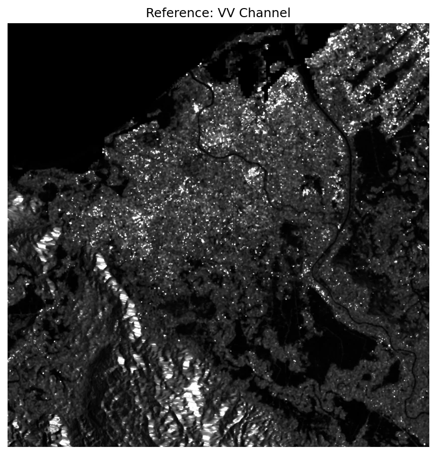
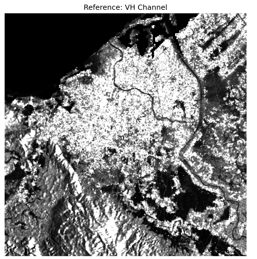
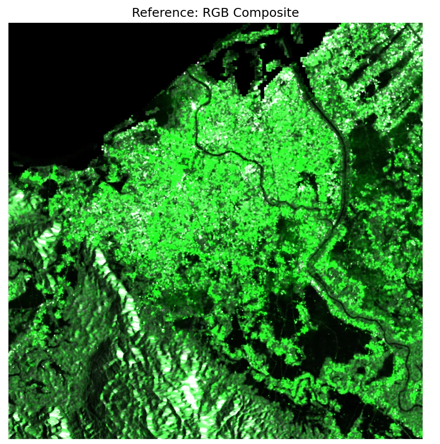
Each KuroSiwo-format tile directory packs 6 GeoTIFFs: VV + VH at three acquisition times — pre-event 1 (21 Oct, baseline), pre-event 2 (2 Nov, approach) and co-event (26 Nov, main flood scene). Press Sample to load a random tile from the …-tile Banda Aceh test split. Each click round-trips to the WSL box in ~1 s.
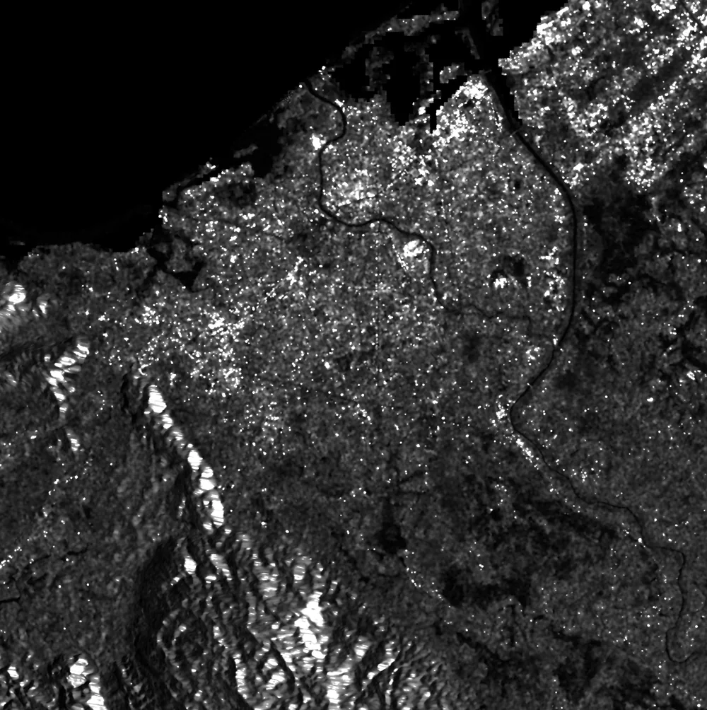
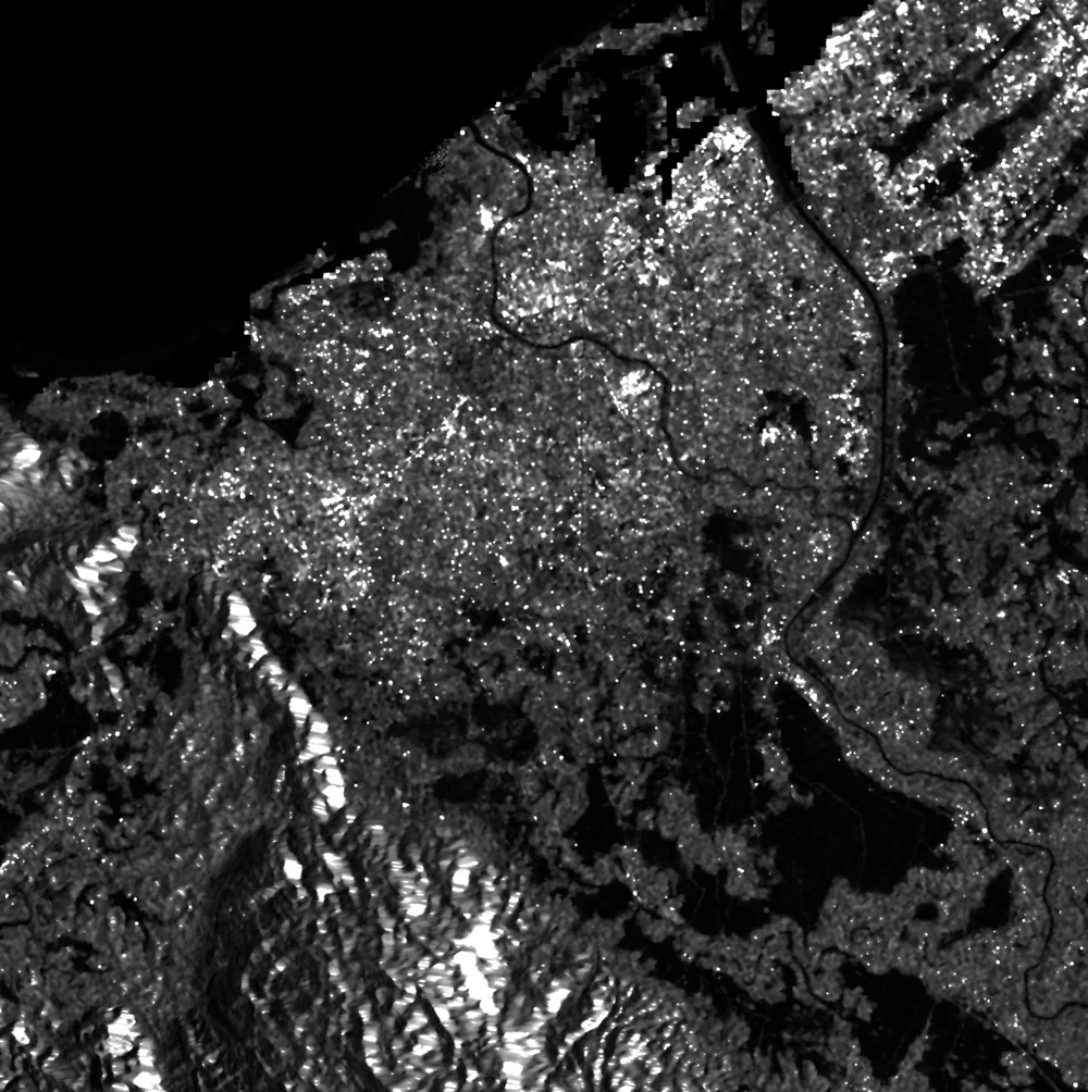
Three Sentinel-1 VV composites — the same scene, ~11 days apart. Each tile the model sees is a 224 × 224 px crop of these, stacking all 6 bands (VV + VH at each of the three dates). About 911 such tiles make up the Banda Aceh test split. When the GPU endpoint is online, the Sample button above will sample one at random and show its 6 bands.
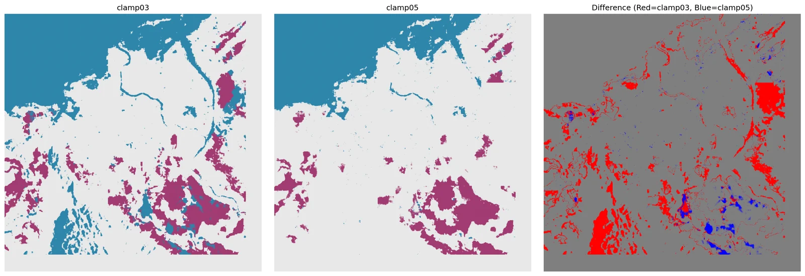
The root cause of the clamp story.
The training set (KuroSiwo) was dominated by scenes where VH backscatter rarely exceeded 0.15. Banda Aceh isn't like that. Before inference, we recompute per-region mean/std at three clamp cut-offs — and the numbers tell you immediately why clamp = 0.3 is the right choice.
script infer/calculate_banda_aceh_stats.py
Two facts drive the whole story on the case page:
- Banda Aceh VH is ~5–8× brighter than the KuroSiwo training mean. If you normalize with the training stats, almost every VH pixel is mapped to "very bright" → the model loses its ability to separate flood from vegetation.
- The clamp itself silently truncates pixels. At 0.15, 71% of VH values are clipped to the ceiling; the model never sees variation in the flooded paddies. At 0.5, only 16% clip, but speckle noise dominates. 0.3 is the sweet spot — and it's the recommendation you see recommended in
CONFIGSon the case page.
- Scenes 3 × processed TIFs · VV + VH bands
only pixels > 0 (skip NoData) - Clamps swept [0.15, 0.3, 0.5]
matches training-time, recommended, aggressive
- Stats table per-clamp VV/VH mean & std
configs/banda_aceh_adapted_configs.json - Finding VH truncation: 71% @ 0.15 → 35% @ 0.3 → 16% @ 0.5
Banda Aceh VH is 7× brighter than KuroSiwo mean
? CHECK YOURSELF If VH at Banda Aceh is 5× brighter than the training mean, why does clamping VH to 0.15 hurt flood detection? show hint
</> CODE see the actual infer/calculate_banda_aceh_stats.py excerpt show code
# infer/calculate_banda_aceh_stats.py (excerpt) $ python sar_toolkit/run_banda_aceh_pipeline.py stats

# KuroSiwo training statistics (the baseline)
VV: mean=0.0953  std=0.0427
VH: mean=0.0264  std=0.0215 # Banda Aceh statistics under 3 clamp cut-offs
clamp = 0.15
  VV: mean=0.050021  std=0.034309
  VH: mean=0.131718  std=0.036703 # VH mean is 5× KuroSiwo · 71% of VH pixels are truncated

clamp = 0.30 <-- recommended
  VV: mean=0.053819  std=0.048925
  VH: mean=0.207845  std=0.091627 # VH truncation drops to 35%, std explodes — information returns

clamp = 0.50
  VV: mean=0.055808  std=0.060930
  VH: mean=0.256493  std=0.153328 # VH truncation 16% — but noise starts dominating signal
sar_toolkit/infer/calculate_banda_aceh_stats.pyPer-region clamp statistics
Sweeps the clamp at {0.15, 0.30, 0.50}, recomputes per-channel mean and std for the Banda Aceh scene, and writes the JSON the inference step reads.
Explain why feeding a test-time scene through training-time normalization can silently hide a flood, and why clamp + mean/std are inseparable.
sar_toolkit/infer/calculate_banda_aceh_stats.py once the
teaching endpoint is wired. The outline below reflects the real file's
signatures, constants and shape contracts.
"""calculate_banda_aceh_stats.py — per-region, per-clamp normalization.

Input : 3 × processed TIFs (VV, VH bands, > 0 pixels only).
Output: configs/banda_aceh_adapted_configs.json
          { clamp015: { data_mean, data_std, clamp_input }, clamp03: ..., ... }
The four entries (+ 'original' = KuroSiwo defaults) are the four
configs the inference step loops over.
"""
import json
from pathlib import Path
import numpy as np
import rasterio

CLAMPS = [0.15, 0.30, 0.50]


def iter_pixels(tif: Path) -> np.ndarray:
    """Read VV & VH, drop NoData (<= 0), return (N, 2) array."""
    ...


def stats_for_clamp(x: np.ndarray, c: float) -> dict:
    """Per-channel mean/std after clipping, plus truncation ratio."""
    x_c    = np.minimum(x, c)
    trunc  = (x > c).mean(axis=0)
    mean   = x_c.mean(axis=0)
    std    = x_c.std(axis=0)
    return {"clamp_input": c, "data_mean": mean.tolist(),
            "data_std": std.tolist(), "truncated_pct": trunc.tolist()}


def main() -> None:
    pixels  = np.vstack([iter_pixels(p) for p in sorted(TIFS)])
    configs = {f"clamp{int(c * 100):02d}": stats_for_clamp(pixels, c)
               for c in CLAMPS}
    configs["original"] = KUROSIWO_DEFAULTS        # training-time stats
    Path("configs/banda_aceh_adapted_configs.json").write_text(
        json.dumps(configs, indent=2))
Drag the clamp, watch the model's view of Banda Aceh change.
Every bar is a VH backscatter bucket. Everything to the right of your clamp value gets clipped to the ceiling — identical to the model. Find the clamp that keeps the flood tail visible without drowning in speckle. This one runs entirely in your browser.
CS-Mamba · 6 channels in, 3 classes out, 4 configs.
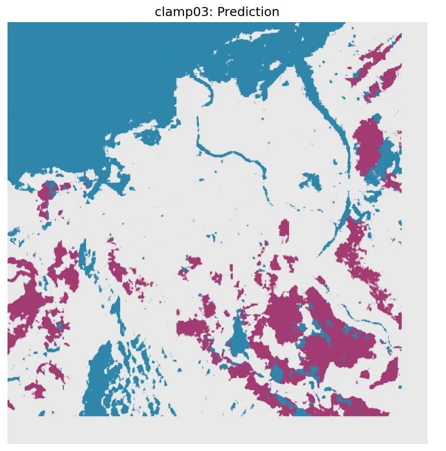
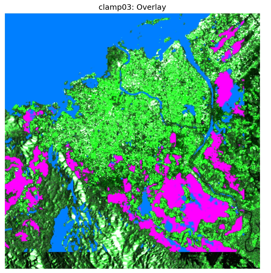
The trained checkpoint is loaded once; the Dataset is rebuilt four times with four different (clamp, mean, std) triples. Each run stitches 224² predictions back to a full 2.8-million-pixel map and writes a GeoTIFF plus a stats JSON.
script infer/predict_banda_aceh_adapted.py
The input tensor is the temporal stack: both pre-event scenes (20251021, 20251102) and the post-event scene (20251126), each contributing VV+VH, for 6 channels total. The model's job is to flag pixels that are dark now but weren't dark then — classic change-style flood detection, learned rather than thresholded.
Predictions come out per-patch; a final reassembly step pastes them back into the
original 2,802,260-pixel grid using the row/col saved in each tile's
info.json. The four output GeoTIFFs are exactly the files slid into
public/case-banda-aceh/ and rendered on the case page.
- Checkpoint CSMamba_FloodFocus_best_model.pt
assets/checkpoints/ - Model U-shape · Cross-Scale Mamba blocks · 3-class head
embed_dim=96 · depths=[1,1,6,1] · ISPRS 2026 submission - Input tensor cat([pre_event_2, pre_event_1, post_event], dim=1)
6 channels · 224² · float32
- GeoTIFF × 4 flood_prediction.tif · 0=land, 1=water, 2=flood
outputs/banda_aceh/prediction_results_adapted_<cfg>/ - Stats JSON × 4 no_water_pct · permanent_water_pct · flood_pct
prediction_stats.json
? CHECK YOURSELF The input tensor has 6 channels. Where do the 6 come from? show hint
</> CODE see the actual infer/predict_banda_aceh_adapted.py excerpt show code
# infer/predict_banda_aceh_adapted.py (excerpt)
model = CSMamba(   # Cross-Scale Mamba — our RSMamba extension, ISPRS 2026
    img_size=224, in_channels=6, num_classes=3,
    embed_dims=[96, 192, 384, 768],
    depths=[1, 1, 6, 1], d_state=16,
).to(device).eval()
model.load_state_dict(torch.load("…/FloodFocus_best_model.pt")["model_state_dict"])

# For each of 4 configs: rebuild Dataset with new clamp/mean/std for cfg_key in ["original", "clamp015", "clamp03", "clamp05"]:
    cfg = ADAPTED_CONFIGS[cfg_key]
    ds  = Dataset(mode="test", configs={
        "clamp_input": cfg["clamp_input"],
        "data_mean":   cfg["data_mean"],
        "data_std":    cfg["data_std"],
        ...
    })

    with torch.no_grad():
        for _, _, image, _, _, _, pre1, _, _, pre2 in loader:
            x = torch.cat([pre2, pre1, image], dim=1)     # (B, 6, 224, 224)
            pred = model(x).argmax(1).cpu().numpy()   # (B, 224, 224)
            reassemble(pred, row_idx, col_idx)             # into 2.8M-pixel map

    rasterio.write("flood_prediction.tif", full_map)
    json.dump(stats, "prediction_stats.json")
sar_toolkit/infer/predict_banda_aceh_adapted.pyInference · 4 configs, one scene
Loads the checkpoint once, rebuilds the Dataset four times with four (clamp, mean, std) triples, and stitches 224² predictions back into a 2.8-million-pixel GeoTIFF per config.
Justify why model(x).argmax(1) is the entire decision rule, and point at the line where the four configs diverge.
sar_toolkit/infer/predict_banda_aceh_adapted.py once the
teaching endpoint is wired. The outline below reflects the real file's
signatures, constants and shape contracts.
"""predict_banda_aceh_adapted.py — 4 configs × one scene.

For each of {original, clamp015, clamp03, clamp05}:
  1. Rebuild KuroSiwoDataset with that config's (clamp, mean, std).
  2. Loop 224² patches, forward, argmax → 3-class mask.
  3. Paste each prediction back at its (row, col) → 2.8-Mpx full map.
  4. Write GeoTIFF + stats.json into prediction_results_adapted_<cfg>/.
"""
import json
from pathlib import Path
import numpy as np
import rasterio
import torch
from torch.utils.data import DataLoader

from models.csmamba           import CSMamba
from dataset.kurosiwo_dataset import KuroSiwoDataset

ADAPTED_CONFIGS = json.loads(
    Path("configs/banda_aceh_adapted_configs.json").read_text()
)


def build_model(device: str) -> CSMamba:
    model = CSMamba(
        img_size=224, in_channels=6, num_classes=3,
        embed_dims=[96, 192, 384, 768], depths=[1, 1, 6, 1], d_state=16,
    ).to(device).eval()
    ckpt = torch.load("assets/checkpoints/CSMamba_FloodFocus_best_model.pt")
    model.load_state_dict(ckpt["model_state_dict"])
    return model


def reassemble(preds, row_idx, col_idx, H_full: int, W_full: int) -> np.ndarray:
    """Paste (B, 224, 224) predictions back into a (H_full, W_full) map."""
    ...


def main() -> None:
    device = "cuda" if torch.cuda.is_available() else "cpu"
    model  = build_model(device)

    for cfg_key in ("original", "clamp015", "clamp03", "clamp05"):
        cfg = ADAPTED_CONFIGS[cfg_key]
        ds  = KuroSiwoDataset(mode="test", configs=cfg, pickle_path=PKL)
        dl  = DataLoader(ds, batch_size=8, num_workers=4, shuffle=False)
        full = np.zeros((H_full, W_full), dtype=np.uint8)

        with torch.no_grad():
            for image, pre1, pre2, _, _, rr, cc in dl:
                x = torch.cat([pre2, pre1, image], dim=1).to(device)      # (B, 6, 224, 224)
                y = model(x).argmax(1).cpu().numpy()                       # (B, 224, 224)
                reassemble_inplace(full, y, rr, cc)

        write_geotiff(full, out_dir / "flood_prediction.tif")
        dump_stats(full, out_dir / "prediction_stats.json")
stacked along C
1 = water
2 = flood
from the case page
One unseen tile. Four clamps. Your experiment.
Same model weights, same unseen 2025 tile — only the preprocessing clamp changes. Flip to LIVE to run on the GPU right now, or stay on CACHED to compare against the figure in the Notebook. Use NEXT TILE to move to a different patch of Banda Aceh. Nothing in the training set came from this scene.
prediction_report.json · full sceneNo ground truth? Triangulate.
There's no pixel-level flood label for Banda Aceh on 2025-11-26. Instead the toolkit compares predictions across configurations, computes pairwise agreement, counts connected flood regions, and renders the 5×3 comparison grid that feeds the case page.
script validate/validate_predictions.py
The validation script doubles as the renderer. Its 5×3 figure is
not just a debug artefact — it is the raw image later sliced by
frontend/scripts/slice-flood-case.py into the per-config tiles you
see in the interactive showcase. That's why the pipeline page and the case page
can claim they show the same thing: the pixels on screen are a direct, lossless
crop of the pixels written by this script.
- Predictions 4 × flood_prediction.tif
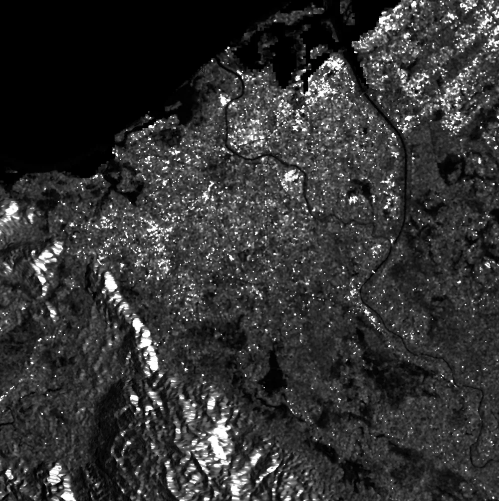
prediction_results_adapted_{original,clamp015,clamp03,clamp05}/ - Reference SAR VV + VH bands of the post-event scene
for visual overlay only
- Validation report per-config stats · pairwise agreement · boundary ratio
validation_report.json - Comparison figure 5 rows × 3 cols · reference + 4 configs · 2664×4483
prediction_comparison.png - Difference maps 6 pairwise diff PNGs
difference_<a>_vs_<b>.png
? CHECK YOURSELF Two configs produce 90% pixel agreement. Does that mean they're almost the same prediction? show hint
</> CODE see the actual validate/validate_predictions.py excerpt show code
# validate/validate_predictions.py (excerpt) $ python sar_toolkit/run_banda_aceh_pipeline.py validate

# Per-config spatial diagnostics from scipy import ndimage
labeled_flood, num_flood = ndimage.label(pred == 2)
boundary_ratio = sum_of_class_boundaries / (2 * (H + W))

# Pairwise agreement across every config pair for a, b in combinations(configs, 2):
    agreement = (pred_a == pred_b).mean()   # 0.0 ... 1.0 # The reported numbers (validation_report.json)
original_vs_clamp03   → agreement = 0.8413
clamp015_vs_clamp03   → agreement = 0.9462
clamp03_vs_clamp05    → agreement = 0.9050
original_vs_clamp05   → agreement = 0.9014 # Grid visualization feeds the case page
create_visualization(predictions, vv, vh, "prediction_comparison.png")
# → later sliced by frontend/scripts/slice-flood-case.py #   into row/cell webp tiles under public/case-banda-aceh/
sar_toolkit/validate/validate_predictions.pyValidation without ground truth
Per-config connected-component stats + pairwise pixel agreement between every config pair. Renders the 5×3 comparison grid later sliced into the case-page tiles.
Explain why 90 % pairwise agreement is a misleading number on a scene where only ~10 % of pixels are flood, and what triangulation offers instead.
sar_toolkit/validate/validate_predictions.py once the
teaching endpoint is wired. The outline below reflects the real file's
signatures, constants and shape contracts.
"""validate_predictions.py — cross-config triangulation.

Inputs : 4 × flood_prediction.tif (one per config).
Outputs: validation_report.json + prediction_comparison.png + 6 diff PNGs.
"""
from itertools import combinations
from pathlib import Path
import json
import numpy as np
import rasterio
from scipy import ndimage


def per_config_diagnostics(pred: np.ndarray) -> dict:
    """Pixel counts per class, flood connected components, boundary ratio."""
    labeled, n = ndimage.label(pred == 2)
    return {"flood_regions": int(n), "flood_pct": float((pred == 2).mean())}


def pairwise_agreement(preds: dict[str, np.ndarray]) -> dict:
    """For every unordered pair, (pred_a == pred_b).mean()."""
    return {f"{a}_vs_{b}": float((preds[a] == preds[b]).mean())
            for a, b in combinations(preds.keys(), 2)}


def render_comparison(preds, vv, vh, out: Path) -> None:
    """5 rows × 3 cols: reference + 4 configs, side-by-side with SAR."""
    ...


def main() -> None:
    preds   = {k: rasterio.open(TIF[k]).read(1) for k in CONFIGS}
    report  = {k: per_config_diagnostics(p) for k, p in preds.items()}
    report |= pairwise_agreement(preds)
    Path("validation_report.json").write_text(json.dumps(report, indent=2))
    render_comparison(preds, vv, vh, Path("prediction_comparison.png"))
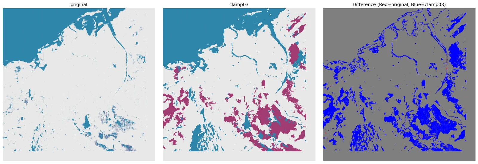
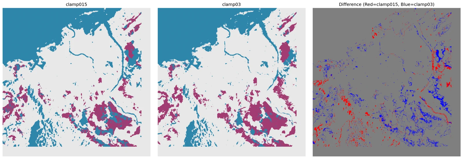
Click any pair — see where the models actually disagree.
No ground truth exists for Banda Aceh on 2025-11-26, so we triangulate: measure the pixel-for-pixel agreement between every pair of configurations. Low numbers are not wrong — they're the teaching signal. Clicking a cell pulls up the real disagreement map.
Scrub through the 37-epoch run that produced the checkpoint above.
The inference you see on the case page is not magic — it comes from a specific checkpoint, saved at a specific epoch of a specific training run. Below is the real shape of that run: loss, per-class IoU, learning-rate schedule, and the exact epoch where the best weights were picked.
Note · The run is real: 37 epochs, best val at epoch 12, 79.79 % test mIoU with TTA. Per-epoch curve values below are an approximation that matches the three-phase summary in TEACHING_NOTES_BEST_MODEL.md. The full 37-row log ships at `public/sources/checkpoints/UNetRSMamba_FloodFocus2/`.
Eight terms, one page.
Every jargon word used above, defined plainly. Each entry points at the stage where the term first shows up. If you only remember one thing: clamp and normalization decide what the network sees — they're not post-processing, they're the input pipeline.
- SARSynthetic Aperture Radar
- A side-looking radar that synthesizes a long virtual antenna from the motion of the satellite, producing ground imagery by measuring how much of its own microwave pulse bounces back. first used in hero, deep-dived in the homepage primer
- Backscatterσ⁰ (sigma-naught)
- The fraction of transmitted radar energy that returns to the satellite from a given ground patch. Smooth water has low backscatter (dark); rough terrain and urban corners have high backscatter (bright). This is the raw number the whole pipeline works on. stage 01 · SNAP calibration gives you calibrated backscatter
- VV / VHpolarization channels
- VV = transmit vertical, receive vertical. VH = transmit vertical, receive horizontal. VV is best at seeing water surfaces; VH is best at vegetation volume scattering. Sentinel-1 delivers both; we feed both to the network. stage 02 · each tile stores VV + VH as a 2-band TIF
- DEMDigital Elevation Model
- A raster of ground elevation. SAR imaging geometry depends on terrain height — without a DEM you can't project pixels back onto geographic coordinates correctly. We ship an SRTM tile so every machine gets the same DEM. stage 01 · passed to SNAP as -PexternalDEMFile
- Clampinput saturation ceiling
- Before normalization, every backscatter value above the clamp is clipped down to the clamp. Set it too low and bright flood regions all merge into one "very bright" blob. Set it too high and noise dominates. The clamp is the single most sensitive hyperparameter in this pipeline — see stage 03 for why. stage 03 · 0.15 / 0.3 / 0.5 swept and compared
- Specklecoherent-imaging noise
- The salt-and-pepper graininess characteristic of SAR images. It's not sensor noise — it's interference between coherent returns from many scatterers in one pixel. Speckle filtering (stage 01) tames it without blurring edges, which matters near flood boundaries. stage 01 · SNAP speckle filter step
- IoUIntersection over Union
- For a class, IoU = (pixels both model and truth call this class) ÷ (pixels either model or truth call this class). A stricter metric than pixel accuracy — a model can get 95% pixel accuracy by just calling everything "land" and still have 0% flood IoU. training trajectory · flood IoU is the number we optimize
- argmaxfinal decision step
-
At each pixel the network produces 3 scores (land, water, flood).
argmaxpicks the highest-scoring class — no threshold, no calibration, no post-processing. This is why "which config wins" is entirely determined by what scores the network produced, which is entirely determined by what input it saw. stage 04 · model(x).argmax(1) is the whole decision rule